

Interrupted time series with a Bayesian structural time series model#
This notebook shows how to use the StateSpaceTimeSeries model with the InterruptedTimeSeries experiment. The model is a Bayesian structural time series (BSTS) built on pymc-extras.statespace: a local level/trend component plus frequency-domain seasonality, estimated with a Kalman filter and smoother. This is the same model family that Google’s CausalImpact [Brodersen et al., 2015] uses to estimate intervention effects from a single time series.
We cover three configurations:
Trend and seasonality only.
Adding control covariates as exogenous regressors.
Automatic covariate selection with a spike-and-slab prior, for the case where you have many candidate control series and want the model to pick the useful ones.
import arviz as az
import matplotlib.pyplot as plt
import numpy as np
import pandas as pd

import causalpy as cp

seed = 42
rng = np.random.default_rng(seed)
sample_kwargs = {
    "draws": 400,
    "tune": 1000,
    "chains": 4,
    "target_accept": 0.95,
    "progressbar": False,
    "random_seed": seed,
}
Simulate data#
We simulate a daily series with a slow upward trend, weekly seasonality, and two control covariates that genuinely drive the outcome (x1, x2). Six more candidate covariates (x3 … x8) are pure noise; they only matter for the covariate selection section. The intervention starts on day 110 and lifts the outcome by 2 units, so we know the true causal effect.
n = 140
dates = pd.date_range(start="2022-01-01", periods=n, freq="D")
treatment_time = dates[110]

trend = 0.02 * np.arange(n)
seasonality = 0.8 * np.sin(2 * np.pi * np.arange(n) / 7)
X = rng.normal(size=(n, 8))
true_effect = np.where(np.arange(n) >= 110, 2.0, 0.0)

y = (
    10
    + trend
    + seasonality
    + 2.0 * X[:, 0]
    - 1.5 * X[:, 1]
    + true_effect
    + rng.normal(0, 0.3, n)
)

df = pd.DataFrame(X, columns=[f"x{i + 1}" for i in range(8)], index=dates).assign(y=y)
df.head()
| x1 | x2 | x3 | x4 | x5 | x6 | x7 | x8 | y | |
|---|---|---|---|---|---|---|---|---|---|
| 2022-01-01 | 0.304717 | -1.039984 | 0.750451 | 0.940565 | -1.951035 | -1.302180 | 0.127840 | -0.316243 | 12.304506 |
| 2022-01-02 | -0.016801 | -0.853044 | 0.879398 | 0.777792 | 0.066031 | 1.127241 | 0.467509 | -0.859292 | 11.892361 |
| 2022-01-03 | 0.368751 | -0.958883 | 0.878450 | -0.049926 | -0.184862 | -0.680930 | 1.222541 | -0.154529 | 12.770824 |
| 2022-01-04 | -0.428328 | -0.352134 | 0.532309 | 0.365444 | 0.412733 | 0.430821 | 2.141648 | -0.406415 | 10.007903 |
| 2022-01-05 | -0.512243 | -0.813773 | 0.615979 | 1.128972 | -0.113947 | -0.840156 | -0.824481 | 0.650593 | 9.873814 |
Trend and seasonality only#
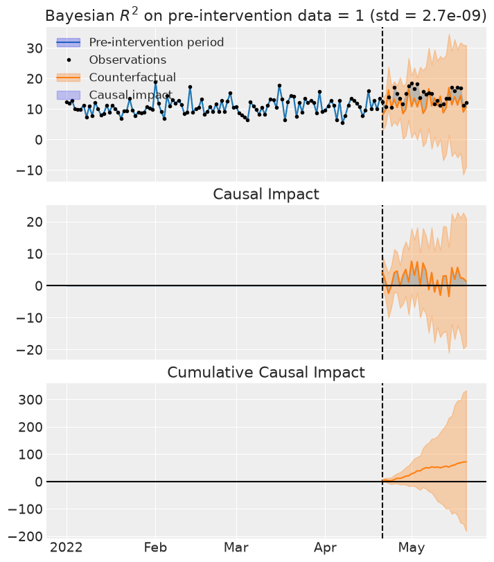
With an intercept-only formula the model uses just its structural components. level_order=2 gives a local linear trend (level and slope), and seasonal_length=7 matches the weekly pattern. The counterfactual for the post-period is a genuine forecast from the Kalman filter, not an in-sample fit.
result_basic = cp.InterruptedTimeSeries(
    data=df[["y"]],
    treatment_time=treatment_time,
    formula="y ~ 1",
    model=cp.pymc_models.StateSpaceTimeSeries(
        level_order=2,
        seasonal_length=7,
        sample_kwargs=sample_kwargs,
    ),
)
fig, ax = result_basic.plot()
                                Model Requirements

  Variable              Shape    Constraints                          Dimensions
 ────────────────────────────────────────────────────────────────────────────────
  initial_level_trend   (2,)                              ('state_level_trend',)
  sigma_level_trend     (2,)     Positive                 ('shock_level_trend',)
  params_freq           (6,)                                     ('state_freq',)
  sigma_freq            ()       Positive                                   None
  P0                    (8, 8)   Positive semi-definite   ('state', 'state_aux')

   These parameters should be assigned priors inside a PyMC model block before
                    calling the build_statespace_graph method.
/home/pablo/micromamba/envs/CausalPy-pymc6/lib/python3.14/site-packages/pymc_extras/statespace/utils/data_tools.py:93: UserWarning: No frequency was specific on the data's DateTimeIndex.
  warnings.warn(NO_FREQ_INFO_WARNING)
Initializing NUTS using jitter+adapt_diag...
Multiprocess sampling (4 chains in 4 jobs)
NUTS: [initial_level_trend, sigma_level_trend, params_freq, sigma_freq, P0_diag]
Sampling 4 chains for 1_000 tune and 400 draw iterations (4_000 + 1_600 draws total) took 108 seconds.
Sampling: [obs]
/home/pablo/micromamba/envs/CausalPy-pymc6/lib/python3.14/site-packages/rich/live.py:260: UserWarning: install
"ipywidgets" for Jupyter support
  warnings.warn('install "ipywidgets" for Jupyter support')
Sampling: [filtered_posterior, filtered_posterior_observed, predicted_posterior, predicted_posterior_observed, smoothed_posterior, smoothed_posterior_observed]
/home/pablo/micromamba/envs/CausalPy-pymc6/lib/python3.14/site-packages/rich/live.py:260: UserWarning: install
"ipywidgets" for Jupyter support
  warnings.warn('install "ipywidgets" for Jupyter support')
Sampling: [forecast_combined]
/home/pablo/micromamba/envs/CausalPy-pymc6/lib/python3.14/site-packages/rich/live.py:260: UserWarning: install
"ipywidgets" for Jupyter support
  warnings.warn('install "ipywidgets" for Jupyter support')
summary_basic = result_basic.effect_summary()
print(summary_basic.text)
During the Post-period (2022-04-21 00:00:00 to 2022-05-20 00:00:00), the response variable had an average value of approx. 14.32. By contrast, in the absence of an intervention, we would have expected an average response of 11.93. The 95% interval of this counterfactual prediction is [2.32, 20.51]. Subtracting this prediction from the observed response yields an estimate of the causal effect the intervention had on the response variable. This effect is 2.39 with a 95% interval of [-6.19, 12.00].

Summing up the individual data points during the Post-period, the response variable had an overall value of 429.74. By contrast, had the intervention not taken place, we would have expected a sum of 357.91. The 95% interval of this prediction is [69.62, 615.33].

The 95% HDI of the effect [-6.19, 12.00] includes zero. The posterior probability of an increase is 0.745. Relative to the counterfactual, the effect represents a 54.01% change (95% HDI [-45.40%, 200.14%]).

This analysis assumes that the relationship between the time-based predictors and the response observed during the pre-intervention period remains stable throughout the post-intervention period. If the formula includes external covariates, it further assumes they were not themselves affected by the intervention. We recommend inspecting model fit, examining pre-intervention trends, and conducting sensitivity analyses (e.g., placebo tests) to support any causal conclusions drawn from this analysis.
Without the covariates the model still finds the effect, but the posterior is wider: the variation that x1 and x2 explain is left in the noise.
Adding control covariates#
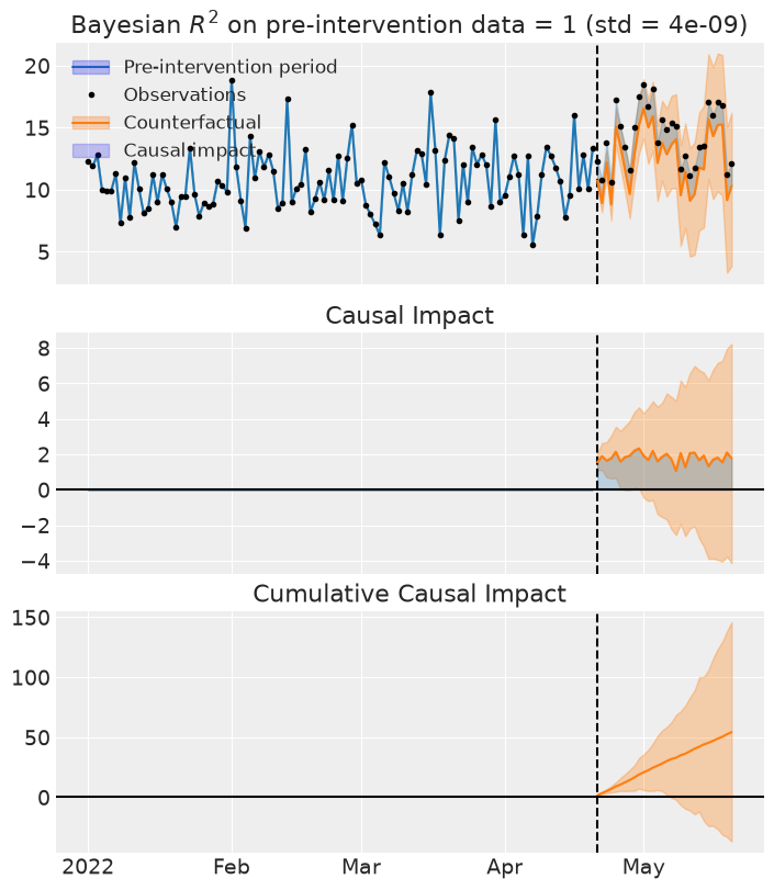
Covariates enter the state-space model through a static regression component, so the counterfactual uses the post-period covariate values when forecasting. Use a 0 + formula: the state-space level already absorbs the intercept, and the model drops a patsy Intercept column (with a warning) if you leave it in.
result_covariates = cp.InterruptedTimeSeries(
    data=df,
    treatment_time=treatment_time,
    formula="y ~ 0 + x1 + x2",
    model=cp.pymc_models.StateSpaceTimeSeries(
        level_order=2,
        seasonal_length=7,
        sample_kwargs=sample_kwargs,
    ),
)
fig, ax = result_covariates.plot()
                                 Model Requirements

  Variable              Shape       Constraints                          Dimensions
 ───────────────────────────────────────────────────────────────────────────────────
  initial_level_trend   (2,)                                 ('state_level_trend',)
  sigma_level_trend     (2,)        Positive                 ('shock_level_trend',)
  params_freq           (6,)                                        ('state_freq',)
  sigma_freq            ()          Positive                                   None
  beta_exog             (2,)                                        ('state_exog',)
  P0                    (10, 10)    Positive semi-definite   ('state', 'state_aux')

  data_exog             (None, 2)   pm.Data                  ('time', 'state_exog')

 These parameters should be assigned priors inside a PyMC model block before calling
                         the build_statespace_graph method.
/home/pablo/micromamba/envs/CausalPy-pymc6/lib/python3.14/site-packages/pymc_extras/statespace/utils/data_tools.py:93: UserWarning: No frequency was specific on the data's DateTimeIndex.
  warnings.warn(NO_FREQ_INFO_WARNING)
Initializing NUTS using jitter+adapt_diag...
Multiprocess sampling (4 chains in 4 jobs)
NUTS: [initial_level_trend, sigma_level_trend, params_freq, sigma_freq, beta_exog, P0_diag]
Sampling 4 chains for 1_000 tune and 400 draw iterations (4_000 + 1_600 draws total) took 139 seconds.
There were 3 divergences after tuning. Increase `target_accept` or reparameterize.
Sampling: [obs]
/home/pablo/micromamba/envs/CausalPy-pymc6/lib/python3.14/site-packages/rich/live.py:260: UserWarning: install
"ipywidgets" for Jupyter support
  warnings.warn('install "ipywidgets" for Jupyter support')
Sampling: [filtered_posterior, filtered_posterior_observed, predicted_posterior, predicted_posterior_observed, smoothed_posterior, smoothed_posterior_observed]
/home/pablo/micromamba/envs/CausalPy-pymc6/lib/python3.14/site-packages/rich/live.py:260: UserWarning: install
"ipywidgets" for Jupyter support
  warnings.warn('install "ipywidgets" for Jupyter support')
Sampling: [forecast_combined]
/home/pablo/micromamba/envs/CausalPy-pymc6/lib/python3.14/site-packages/rich/live.py:260: UserWarning: install
"ipywidgets" for Jupyter support
  warnings.warn('install "ipywidgets" for Jupyter support')
az.summary(
    result_covariates.idata,
    var_names=["beta_exog"],
    kind="stats",
    ci_kind="hdi",
    ci_prob=0.94,
)
| mean | sd | hdi94_lb | hdi94_ub | |
|---|---|---|---|---|
| beta_exog[x1] | 2 | 1.4 | -0.84 | 4.6 |
| beta_exog[x2] | -1.5 | 1.4 | -4.3 | 1.3 |
summary_covariates = result_covariates.effect_summary()
print(summary_covariates.text)
During the Post-period (2022-04-21 00:00:00 to 2022-05-20 00:00:00), the response variable had an average value of approx. 14.32. By contrast, in the absence of an intervention, we would have expected an average response of 12.52. The 95% interval of this counterfactual prediction is [9.49, 15.89]. Subtracting this prediction from the observed response yields an estimate of the causal effect the intervention had on the response variable. This effect is 1.81 with a 95% interval of [-1.57, 4.84].

Summing up the individual data points during the Post-period, the response variable had an overall value of 429.74. By contrast, had the intervention not taken place, we would have expected a sum of 375.53. The 95% interval of this prediction is [284.57, 476.85].

The 95% HDI of the effect [-1.57, 4.84] includes zero. The posterior probability of an increase is 0.891. Relative to the counterfactual, the effect represents a 16.49% change (95% HDI [-11.39%, 48.66%]).

This analysis assumes that the relationship between the time-based predictors and the response observed during the pre-intervention period remains stable throughout the post-intervention period. If the formula includes external covariates, it further assumes they were not themselves affected by the intervention. We recommend inspecting model fit, examining pre-intervention trends, and conducting sensitivity analyses (e.g., placebo tests) to support any causal conclusions drawn from this analysis.
The regression coefficients recover the true values (2.0 and -1.5), and the effect estimate tightens.
Automatic covariate selection#
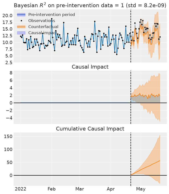
When you have many candidate control series, a spike-and-slab prior on the regression coefficients lets the model decide which ones matter, mirroring CausalImpact’s approach. Pass vs_prior_type="spike_and_slab" and give the model all candidates.
Read the posterior inclusion probabilities as a relative ranking of the candidates rather than as calibrated probabilities. Under this prior the beta_exog point estimates shrink toward zero (the state-space initial covariance lets the regression states drift from the parameter), but the counterfactual forecast comes from the smoothed states and is not affected.
result_selection = cp.InterruptedTimeSeries(
    data=df,
    treatment_time=treatment_time,
    formula="y ~ 0 + " + " + ".join(f"x{i + 1}" for i in range(8)),
    model=cp.pymc_models.StateSpaceTimeSeries(
        level_order=2,
        seasonal_length=7,
        sample_kwargs=sample_kwargs,
        vs_prior_type="spike_and_slab",
    ),
)
fig, ax = result_selection.plot()
                                 Model Requirements

  Variable              Shape       Constraints                          Dimensions
 ───────────────────────────────────────────────────────────────────────────────────
  initial_level_trend   (2,)                                 ('state_level_trend',)
  sigma_level_trend     (2,)        Positive                 ('shock_level_trend',)
  params_freq           (6,)                                        ('state_freq',)
  sigma_freq            ()          Positive                                   None
  beta_exog             (8,)                                        ('state_exog',)
  P0                    (16, 16)    Positive semi-definite   ('state', 'state_aux')

  data_exog             (None, 8)   pm.Data                  ('time', 'state_exog')

 These parameters should be assigned priors inside a PyMC model block before calling
                         the build_statespace_graph method.
/home/pablo/micromamba/envs/CausalPy-pymc6/lib/python3.14/site-packages/pymc_extras/statespace/utils/data_tools.py:93: UserWarning: No frequency was specific on the data's DateTimeIndex.
  warnings.warn(NO_FREQ_INFO_WARNING)
Initializing NUTS using jitter+adapt_diag...
Multiprocess sampling (4 chains in 4 jobs)
NUTS: [initial_level_trend, sigma_level_trend, params_freq, sigma_freq, pi_beta_exog, beta_exog_raw, gamma_beta_exog_u, P0_diag]
Sampling 4 chains for 1_000 tune and 400 draw iterations (4_000 + 1_600 draws total) took 586 seconds.
The rhat statistic is larger than 1.01 for some parameters. This indicates problems during sampling. See https://arxiv.org/abs/1903.08008 for details
Sampling: [obs]
/home/pablo/micromamba/envs/CausalPy-pymc6/lib/python3.14/site-packages/rich/live.py:260: UserWarning: install
"ipywidgets" for Jupyter support
  warnings.warn('install "ipywidgets" for Jupyter support')
Sampling: [filtered_posterior, filtered_posterior_observed, predicted_posterior, predicted_posterior_observed, smoothed_posterior, smoothed_posterior_observed]
/home/pablo/micromamba/envs/CausalPy-pymc6/lib/python3.14/site-packages/rich/live.py:260: UserWarning: install
"ipywidgets" for Jupyter support
  warnings.warn('install "ipywidgets" for Jupyter support')
Sampling: [forecast_combined]
/home/pablo/micromamba/envs/CausalPy-pymc6/lib/python3.14/site-packages/rich/live.py:260: UserWarning: install
"ipywidgets" for Jupyter support
  warnings.warn('install "ipywidgets" for Jupyter support')
inclusion = result_selection.model.get_inclusion_probabilities()
inclusion.index = [f"x{i + 1}" for i in range(8)]

fig, ax = plt.subplots()
inclusion["prob"].sort_values().plot.barh(ax=ax)
ax.axvline(0.5, color="k", linestyle="--", linewidth=1)
ax.set(xlabel="Posterior inclusion probability", title="Covariate selection");
The two real predictors rank clearly above the noise covariates.
PyMC reports an rhat above 1.01 for this model. Spike-and-slab posteriors are multimodal by construction, so chains can disagree about individual coefficients. Read the inclusion probabilities rather than the coefficient summaries here, and raise tune and draws if you need tighter per-coefficient estimates.
Notes#
The model needs a
pandas.DatetimeIndexand a single treated unit.Missing values in the outcome are handled natively by the Kalman filter; covariates must be complete.
Override priors per parameter with the
priorsargument, e.g.priors={"sigma_freq": Prior("HalfNormal", sigma=1)}.
References#
Kay H. Brodersen, Fabian Gallusser, Jim Koehler, Nicolas Remy, and Steven L. Scott. Inferring causal impact using bayesian structural time-series models. The Annals of Applied Statistics, 9(1):247–274, 2015.